ADC/SS-PCM at glance! - part two

This post is a follow up on my last post, in which I discussed the accuracy of the ADC/SS-PCM approach for a number of push-pull systems. So if you haven't read part one yet, please do so before you continue.

Part one ended with the finding that solvent effects were significantly over-estimated for the type of molecule under investigation. More specifically, the shift of the fluorescence energy between non-polar cyclohexane (chx) and polar acetonitrile (acn) solution calculated with ADC(2)/SS-PCM was exactly twice as large as the experimental numbers - for almost all of the systems. Even more surprisingly, the theoretically ill-defined one-shot approach (quick reminder: one-shot means that I use the result from the first step of the solvent-field iterations) seemingly provides a much better agreement with the experiment than the converged solvent-field:

I ended that first part with the promise to explain why I'm sure that this is a coincidence, what/how we can learn from it, and what underlying cause is responsible for the problem. So let's go:

Why is the fact that the calculation is of by almost exactly a factor of two in 5 out of 6 molecules for which there is experimental data a (more or less) lucky coincidence and not a simple bug (factor of two missing somewhere in the code)? I think there is a number of reasons, the most important of which is the crude level of theory that has been applied. First of all, we've used the same gas-phase optimized omega-PBE/6-31+g* geometries for all of the ADC/SS-PCM calculations. Hence, we are neglecting all structural effects of the the solvent stabilization. While this is probably okay for the weaker solvents (chx), it will most certainly affect the results in acn and thus modulate the chx to acn shifts. Secondly, the ADC calculations are carried out with a really small, non-polarized split-valence basis set (def2-SV), which is simply to limit the computational demands for these already quite large molecules. In calculations exploring this issue for ZMSO2-14 with the partially polarized def2-SV(P) and def2-SVP, the calculated shifts decreased by about 0.1 eV and the suspicious factor of two (actually 1.97) becomes a less suspicious factor of 1.87. (Mind that def2-SVP is still a rather small basis). Thirdly, the molecules are all very similar, such that it is not really surprising to find the same systematic error for 5 out of 6 of them. So far, I have never observed something even remotely similar for any of the other (push-pull) systems I have computed with this method. After all, I'm convinced that the factor of two is a coincidence.

But if it is a coincidence, what can we learn from it?

The fact that the error is so suspiciously constant just means that it is very systematic. Systematic errors are much nicer than statistic ones, because its very straightforward to correct them. In this particular case, the correction is simply dividing the shifts by two. Inspecting the plot of the results above, you will find that the results from the converged solvent field divided by two (green line) reproduce the experiment even better than the one-shot results. Or in other words: Although the one-shot approach is much closer to the experiment in absolute numbers, the converged results follow the experimental trend more closely, i.e., their statistical error is smaller. The good news is that after all, this shows that the solvent-field iterations indeed improve the results compared to the one-shot approach. This was just difficult to see because of a large systematic error. Eventually, we are left with the remaining question:

What is the reason for this large systematic error?

As I already mentioned on a number of occasions, ADC(2) seems to over-stabilize states with large density shifts, such as CT states. I think this due to too large orbital-relaxation effects. Orbital relaxation is the response of the molecular density to the primary electron transfer during an excitation. While this is quite difficult to explain in words, it is quite apparent from a comparison of the the electron and hole densities of an excitation (initial electron transfer) to the total attachment and detachment densities (including orbital relaxation). Here I have calculated and visualized all of these for  ZMSO2-14:

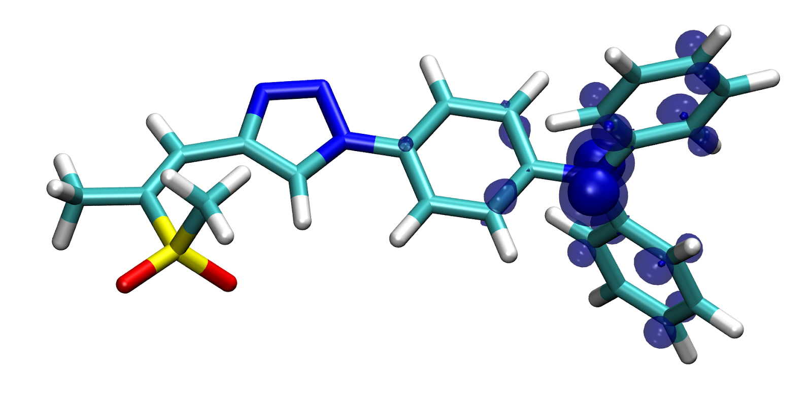
While the electron (top left) and hole (top right) densities appear to be rather independent (positions and sizes of the visible blobs are uncorrelated), they show that in this excited state an electron from the nitrogen lone-pair is excited into a pi* orbital. The attachment (bottom left) and detachment (bottom right) densities are, in contrast to that, clearly not independent, but correlated. Wherever there is a positive contribution in the hole/attachment density (e.g. the extra electron in the pi-system in the left part of the molecule), one can find negative blue (orbital-relaxation) contributions at the same place in the sigma system in the detachment density. Vice versa, wherever density vanishes, e.g. from the nitrogen lone-pair, there are positive relaxation contributions in the attachment density, which are clearly not there in the primary electron density. This response of the density to the initially excited electron/excitation-hole is exactly what I understand to be orbital relaxation. To have an even more intuitive picture, I should probably go ahead and plot just the difference between the electron/hole and  attachment/detachment densities, but for now the pictures above must suffice.

However, while these pictures are nice to illustrate the effect, one needs a more quantitative measure to see how strong orbital relaxation is in these molecules, and to compare it to other molecules. For this purpose, its advisable to look at the so-called promotion numbers, which can be seen as integrals over the attachment/detachment densities, or in other words the number of electrons that is involved in/shifted around during the excitation. A typical locally excited state would have a promotion number of around 1.5, meaning that in addition to the initially excited electron, a total of 0.5 electrons make up the orbital relaxation. For charge-transfer states which do in general have stronger orbital relaxation (because more charge is shifted around), these numbers are closer to or maybe even larger than two. Let us now take a look how the promotion numbers of ZMS-14 and ZMSO2-14 evolve during the solvent-field iterations in chx, diethylether (eth), dichloromethane (dcm) and acn (please focus only on the reddish and blueish lines for now):

Plot of the promition numbers of the weak and strong push-pull systems ZMS-14 and ZMSO2-14 as well as the TADF chromophore termed F1 calculated during the solvent-field iterations in chx, eth, dcm and acn at the ADC(2)/SS-PCM/SV level of theory. While the iterations in chx converge in 4-5 steps (here including the vertical excitation as step 1), it takes 6-11 steps to converge in the polar solvent acn. Beginning at roughly the same value of 2 in all solvents for ZMS and ZMSO2-14, the promotion numbers hardly change for ZMS in chx, while there is a large increase to about 2.6 for in ZMSO2 in the polar solvents. For F1, the changes are much smaller and the promotion numbers are virtually unaffected by the solvent-field.

Apparently, there is a significant increase of the promotion numbers and thus the amount of orbital relaxation during the solvent-field iterations in polar solvents, even for the weaker push-pull systems. The promotion numbers increase to unphysically large values of 2.5 and larger for ZMSO2-14 in polar solvents and reach 2.2 even in chx. In general, I was surprised that the promotion number change at all during the iterations, which is something I have never observed before. I have investigated a number of large push-pull systems designed for TADF with the very same methodology and small systems such as DMABN with ADC2 and ADC3/SS-PCM, for which I obtained much better agreement for the calculated chx to acn shifts. Also, in all of these examples, the promotion numbers hardly ever change during the iterations, as evident from the the representative example termed F1 shown in the figure above as greenish lines (the molecule is taken form this article).

A similar problem with unphysically large promotion numbers accommodated by faulty excitation energies at the ADC(2) level of theory was reported by my friend and colleague Felix in an investigation of iridium complexes. In his case, the problem appeared in the gas-phase calculation and was corrected at the ADC(3) level of theory.

After all, I tend to think this is an ADC(2) problem that is amplified/unveiled during the solvent-field iterations.  Consequently, one should carefully check the evolution of the promotion numbers during the solvent field iterations (they can be obtained by activating "state_analysis = true" and "nto_pairs = 2" in the $rem block of the input file). If there are large changes, one should be extra careful with the results of the method.