New Website

Dear Reader

After years of misusing this blog for a website, I finally made a real website for myself. You can find it here (www.janmewes.de) since I moved the redirect today. 

Have some nice and healthy holidays and a happy new year!
Jan

Dr. Jan-Michael Mewes

Recent Publications: (all)

Schmitz, Schwerdtfeger, Grimme, Mewes, JACS, 2021/22 (just accepted)
“It's Complicated: On Relativistic Effects and Periodic Trends in the Melting and Boiling Points of the Group 11 Coinage Metals”

Kunze, Hansen, Grimme, Mewes, JPCL, 2021 
“PCM-ROKS for the Description of Charge-Transfer States in Solution: Singlet-Triplet Gaps with Chemical Accuracy from Open-Shell Self-Consistent Reaction-Field Calculations”

Mewes, Hansen, Grimme, Angewandte, 2021
“Comment on ‘The Nature of Chalcogen‐Bonding‐Type Tellurium–Nitrogen Interactions’: Fixing the Description of Finite-Temperature Effects Restores the Agreement Between Experiment and Theory”
(Open Access)

Mewes, Schwerdtfeger, Angewandte, 2021
Exclusively Relativistic: Periodic Trends in the Melting and Boiling Points of Group 12
(Open Access, auch auf Deutsch)

Grimme, Hansen, Ehlert, Mewes, JCP, 2021
r²SCAN-3c: A "Swiss Army Knife" Composite Electronic-Structure Method 

Mewes, Smits, PCCP, 2020
Accurate Elemental Boiling Points From First Principles

Scholz, Massoth, Bursch, Mewes, Hetzke, Wolf, Bolte, Lerner, Grimme, Wagner, JACS, 2020:

BNB-Doped Phenalenyls: Modular Synthesis, Optoelectronic Properties, and One-Electron Reduction

Smits, Mewes, Jerabek, Schwerdtfeger, Angewandte, 2020:

Oganesson: A Noble-Gas Element that is Neither Noble Nor a Gas
(Open Access)

Caldeweyher, Mewes, Ehlert, Grimme, PCCP, 2020:
Extension and evaluation of the D4 London-dispersion correction for periodic solids
(HOT Article)

Mewes, Smits, Kresse, Schwerdtfeger, Angewandte, 2019:
Copernicium: A Relativistic Noble Liquid
(Open Access)

Mewes, Smits, Jerabek, Schwerdtfeger, Angewandte, 2019:
Oganesson is a Semiconductor: On the Relativistic Band-Gap Narrowing in the Heaviest Noble-Gas Solids
(Hot Paper, Open Access, auf Deutsch) 

Trombach, Ehlert, Grimme, Schwerdtfeger, Mewes, PCCP, 2019:
Exploring the chemical nature of super-heavy main-group elements by means of efficient plane-wave density-functional theory
(HOT Article, Frontcover)

Mewes, PCCP, 2018: 
Modeling TADF in organic emitters requires careful consideration of the environment and going beyond the Franck–Condon approximation

(HOT Article) 

Professional: 

Jan 2021 – current

Scientific Consultant, Lanthanoid-based OLEDs
beeOLED GmbH, Dresden

Jun 2019 – current

Postdoc/Senior Researcher (one-year returning Scholarship, AvH) 
with Prof. Stefan Grimme,
Mulliken-Center for Theoretical Chemistry, Bonn

Sep 2016 – May 2019 

Feodor-Lynen Postdoc (Scholarship of the Alexander-von-Humboldt Foundation)
with Prof. Peter Schwerdtfeger,
New Zealand Institute for Advanced Study (NZIAS), Auckland

Mar 2015 – Aug 2016 

Postdoc (Scholarship of HGS Mathcomp)
with Prof. Andreas Dreuw
Interdisciplinary Center for Scientific Computing, Heidelberg

Education:

Oct 2010 – Feb 2015
Ph.D. in Theoretical Chemistry
with Prof. Andreas Dreuw,
Interdisciplinary Center for Scientific Computing (IWR), Heidelberg,
Fellow of the HGS MathComp
Thesis: „Development and Application of Methods for the Description of Photochemical Processes in Condensed Phase“.

Oct 2008 – Sep 2010
Master of Science in Chemistry,
with Prof. Andreas Dreuw,
Goethe-University, Frankfurt
Thesis: „The Mechanism of Photodecarboxylation of Nitrophenylacetate and the Implications for Ortho-Nitrobenzyl Caged Compounds“.

Oct 2005 – Sep 2008
Bachelor of Science in Chemistry,
with Prof. Andreas Dreuw,
Goethe-University, Frankfurt 

Thesis (German): „Energietransfer in Bakteriellen Lichtsammelkomplexen“.

the final update

After almost three years without a new post, I have to admit that as an early-career scientist and father of two (1 and 4), the time for running a research blog is very limited. Thus, I will turn this website into a somewhat more static source of information.

so long,
Jan

ADC/SS-PCM at glance! - part two

This post is a follow up on my last post, in which I discussed the accuracy of the ADC/SS-PCM approach for a number of push-pull systems. So if you haven't read part one yet, please do so before you continue.

Part one ended with the finding that solvent effects were significantly over-estimated for the type of molecule under investigation. More specifically, the shift of the fluorescence energy between non-polar cyclohexane (chx) and polar acetonitrile (acn) solution calculated with ADC(2)/SS-PCM was exactly twice as large as the experimental numbers - for almost all of the systems. Even more surprisingly, the theoretically ill-defined one-shot approach (quick reminder: one-shot means that I use the result from the first step of the solvent-field iterations) seemingly provides a much better agreement with the experiment than the converged solvent-field:

I ended that first part with the promise to explain why I'm sure that this is a coincidence, what/how we can learn from it, and what underlying cause is responsible for the problem. So let's go:

Why is the fact that the calculation is of by almost exactly a factor of two in 5 out of 6 molecules for which there is experimental data a (more or less) lucky coincidence and not a simple bug (factor of two missing somewhere in the code)? I think there is a number of reasons, the most important of which is the crude level of theory that has been applied. First of all, we've used the same gas-phase optimized omega-PBE/6-31+g* geometries for all of the ADC/SS-PCM calculations. Hence, we are neglecting all structural effects of the the solvent stabilization. While this is probably okay for the weaker solvents (chx), it will most certainly affect the results in acn and thus modulate the chx to acn shifts. Secondly, the ADC calculations are carried out with a really small, non-polarized split-valence basis set (def2-SV), which is simply to limit the computational demands for these already quite large molecules. In calculations exploring this issue for ZMSO2-14 with the partially polarized def2-SV(P) and def2-SVP, the calculated shifts decreased by about 0.1 eV and the suspicious factor of two (actually 1.97) becomes a less suspicious factor of 1.87. (Mind that def2-SVP is still a rather small basis). Thirdly, the molecules are all very similar, such that it is not really surprising to find the same systematic error for 5 out of 6 of them. So far, I have never observed something even remotely similar for any of the other (push-pull) systems I have computed with this method. After all, I'm convinced that the factor of two is a coincidence.

But if it is a coincidence, what can we learn from it?

The fact that the error is so suspiciously constant just means that it is very systematic. Systematic errors are much nicer than statistic ones, because its very straightforward to correct them. In this particular case, the correction is simply dividing the shifts by two. Inspecting the plot of the results above, you will find that the results from the converged solvent field divided by two (green line) reproduce the experiment even better than the one-shot results. Or in other words: Although the one-shot approach is much closer to the experiment in absolute numbers, the converged results follow the experimental trend more closely, i.e., their statistical error is smaller. The good news is that after all, this shows that the solvent-field iterations indeed improve the results compared to the one-shot approach. This was just difficult to see because of a large systematic error. Eventually, we are left with the remaining question:

What is the reason for this large systematic error?

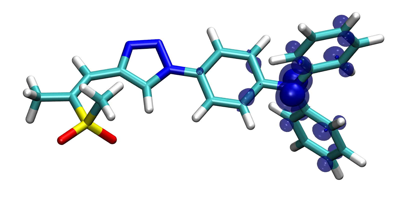
As I already mentioned on a number of occasions, ADC(2) seems to over-stabilize states with large density shifts, such as CT states. I think this due to too large orbital-relaxation effects. Orbital relaxation is the response of the molecular density to the primary electron transfer during an excitation. While this is quite difficult to explain in words, it is quite apparent from a comparison of the the electron and hole densities of an excitation (initial electron transfer) to the total attachment and detachment densities (including orbital relaxation). Here I have calculated and visualized all of these for  ZMSO2-14:

While the electron (top left) and hole (top right) densities appear to be rather independent (positions and sizes of the visible blobs are uncorrelated), they show that in this excited state an electron from the nitrogen lone-pair is excited into a pi* orbital. The attachment (bottom left) and detachment (bottom right) densities are, in contrast to that, clearly not independent, but correlated. Wherever there is a positive contribution in the hole/attachment density (e.g. the extra electron in the pi-system in the left part of the molecule), one can find negative blue (orbital-relaxation) contributions at the same place in the sigma system in the detachment density. Vice versa, wherever density vanishes, e.g. from the nitrogen lone-pair, there are positive relaxation contributions in the attachment density, which are clearly not there in the primary electron density. This response of the density to the initially excited electron/excitation-hole is exactly what I understand to be orbital relaxation. To have an even more intuitive picture, I should probably go ahead and plot just the difference between the electron/hole and  attachment/detachment densities, but for now the pictures above must suffice.

However, while these pictures are nice to illustrate the effect, one needs a more quantitative measure to see how strong orbital relaxation is in these molecules, and to compare it to other molecules. For this purpose, its advisable to look at the so-called promotion numbers, which can be seen as integrals over the attachment/detachment densities, or in other words the number of electrons that is involved in/shifted around during the excitation. A typical locally excited state would have a promotion number of around 1.5, meaning that in addition to the initially excited electron, a total of 0.5 electrons make up the orbital relaxation. For charge-transfer states which do in general have stronger orbital relaxation (because more charge is shifted around), these numbers are closer to or maybe even larger than two. Let us now take a look how the promotion numbers of ZMS-14 and ZMSO2-14 evolve during the solvent-field iterations in chx, diethylether (eth), dichloromethane (dcm) and acn (please focus only on the reddish and blueish lines for now):

Plot of the promition numbers of the weak and strong push-pull systems ZMS-14 and ZMSO2-14 as well as the TADF chromophore termed F1 calculated during the solvent-field iterations in chx, eth, dcm and acn at the ADC(2)/SS-PCM/SV level of theory. While the iterations in chx converge in 4-5 steps (here including the vertical excitation as step 1), it takes 6-11 steps to converge in the polar solvent acn. Beginning at roughly the same value of 2 in all solvents for ZMS and ZMSO2-14, the promotion numbers hardly change for ZMS in chx, while there is a large increase to about 2.6 for in ZMSO2 in the polar solvents. For F1, the changes are much smaller and the promotion numbers are virtually unaffected by the solvent-field.

Apparently, there is a significant increase of the promotion numbers and thus the amount of orbital relaxation during the solvent-field iterations in polar solvents, even for the weaker push-pull systems. The promotion numbers increase to unphysically large values of 2.5 and larger for ZMSO2-14 in polar solvents and reach 2.2 even in chx. In general, I was surprised that the promotion number change at all during the iterations, which is something I have never observed before. I have investigated a number of large push-pull systems designed for TADF with the very same methodology and small systems such as DMABN with ADC2 and ADC3/SS-PCM, for which I obtained much better agreement for the calculated chx to acn shifts. Also, in all of these examples, the promotion numbers hardly ever change during the iterations, as evident from the the representative example termed F1 shown in the figure above as greenish lines (the molecule is taken form this article).

A similar problem with unphysically large promotion numbers accommodated by faulty excitation energies at the ADC(2) level of theory was reported by my friend and colleague Felix in an investigation of iridium complexes. In his case, the problem appeared in the gas-phase calculation and was corrected at the ADC(3) level of theory.

After all, I tend to think this is an ADC(2) problem that is amplified/unveiled during the solvent-field iterations.  Consequently, one should carefully check the evolution of the promotion numbers during the solvent field iterations (they can be obtained by activating "state_analysis = true" and "nto_pairs = 2" in the $rem block of the input file). If there are large changes, one should be extra careful with the results of the method.

ADC/SS-PCM at glance? - part one

Dear colleagues,

 

in the framework of a recent project published in this article, I for the first time had the chance to systematically study the performance of ADC/SS-PCM for a group of click-chemistry generated molecules with varying charge-transfer character in their emitting excited state.
The common motif of these molecule is that they consist of an electron-pushing triphenylamin group (right side of the molecule in the figure below) and an electron-pulling group (left side), whose strength can be modulated by oxidizing the contained sulphur atom. In the lowest excited singlet state of all of these systems, an electron is excited from the electron-pushing triphenylamine to the electron pulling part of the molecule. While the excitation-hole turned out to be essentially identical in all of these systems and all solvents, the location and structure of the excited electron differed significantly depending on the molecule and environment.
The figure below shows the structures of the molecules as well as the location of the excited electron computed at the ADC2/SS-PCM/SV level of theory for the non-polar solvent cyclohexane on the left and for the polar solvent acetonitrile in the right.

Since the discussion of the performance of the methodology was (as usual) quite brief in the article, I will share some more methodological insights here and in the following posts.
The central observation, which also made it into the paper, was that the solvent effects are systematically overestimated for this group of molecules, leading to too low emission energies in polar solvents (here acetonitrile, ACN). In the non-polar solvent cyclohexane (CHX) the error seems to cancel out with the systematic overestimation of the emission energies by the quantum-chemical method (ADC2 with a small, non-polarized split-valence basis), leading to a very reasonable agreement. 

Something that we only mentioned but did not show in the article was that the spin-opposite scaled variant of ADC(2), SOS-ADC(2) [short: SOS(2)] improves on this systematic error. After the article was published I took a closer look at this and recomputed all of the numbers also with SOS(2). Turns out this method pretty much nails the emission energies in ACN, with those in CHX getting a little worse:

Fluorescence energies of a series of molecules calculated with ADC(2) and SOS-ADC(2)/SS-PCM/SV using TD-uPBE/6-31+G(d) geometries. Geometry optimizations were conducted in the gas phase, i.e., without any solvent model.

While these trends are most certainly interesting to know for future investigations (use SOS-ADC/SV for polar solvents and ADC/SV for non-polar ones), the question that remains is if this systematic overestimation of the solvent-stabilization is due to A) the quantum-chemical methodology, B) the solvent-model, C) the nature of these molecules or D) a combination of all three. 

Speaking for A) is that I have observed before how ADC(2) yields too low energies for charge-transfer states compared to locally excited states. Since in this case the picture was very consistent, including the fact that the problem is corrected by ADC(3), I'm pretty confident that A) contributes at least to some extent. The question that really bothers me, however, is if B) is also the case, because so far, I am pretty sure that the self-consistent treatment of solvent polarization is the one and only physically correct way to do it. You can find my arguments for that in the respective article (same as above).

To further look into the issue, let us eliminate the inherent error of the quantum-chemical methodology as far as possible by looking at the CHX to ACN shifts in the emission energy. Let us furthermore include the emission energies from the first solvent-field iteration in the comparison, i.e. the ones calculated with the solvent field obtained for the excited-state computed in the relaxed ground-state solvent field (ptSS-calculation).

Seeing this plot for the first time literally shocked me. The agreement of the one-shot approach with the experimental data is so apparent and convincing that I immediately starting looking for the fundamental flaw in the self-consistent approach. The latter apparently overestimated the shifts by about a factor of two. Did I say about? For ADC(2), its pretty much exactly a factor of two:

Can this be a coincidence? Exactly a factor of two? The lines are pretty much on top of each other. Yet, I'm pretty sure (as sure as it gets for a scientist) that this is indeed a coincidence, for a number of convincing reasons, which I will elaborate in the next post. And the best thing will be, that we can still learn from this coincidence!

So long,

Jan

Boron-substituted aromatics - part two: thermochemical calculations

In my last post I described how I calculated vibrationally resolved UV/vis absorption spectra for a couple of boronaromatics and their acetonitrile (ACN) adducts and how this helped to resolve the mystery of their odd solvatochromism (solvent dependent absorption spectra). The one question that remained open was: Do DBI and DBA exclusively form 1:1 monoadducts with ACN or also the 1:2 diadducts? Since the latter are predicted to have essentially no absorption in the relevant spectral range, i.e., between 300 and 700 nm, I could neither confirm nor exclude their formation.

To answer this question, I started to conduct what was planned as a "brief" thermochemical analysis of formation of the respective mono- and diadducts. However, since the first results were inconclusive the I ended up employing a hierarchy of methods of increasing sophistication (and computational demand), which only eventually (at the very highest level of theory) cumulated in a good enough agreement with the experimental observations. I think the convergence of the results with respect to level of theory and employed basis-sets is quite instructive (without having much experience in quantum-thermochemistry), but at the same time too long and theoretical to be included in the article, and hence provides a nice topic for this blog. Lets get to it!

The initial plan was to just collect and investigate the results from the calculations I had already conducted to model the vibrationally resolved spectra. These include all optimizations and normal-mode analyses for naked DBI, DBA and DBP as well as their monoadducts and trans-diadducts, such that solely the respective calculations for ACN were missing. Having completed the latter and putting together all the numbers (computed at the same level of theory as the vibronic spectra, i.e., B3LYP-D3BJ/SVP) afforded the following picture:

Thermochemical data for the formation of the ACN mono- and diadduct of DBI, DBA and DBP (only trans-diadduct of DBI is shown) calculated at the B3LYP-D3BJ/SVP level of theory (using the COSMO solvation model to mimic the influence of the solvent ACN here and in all of the following results). The leftmost value termed "electronic" is computed from the electronic energies only. "ZPE" additionally includes the energy changes due to zero-point vibrations, which make the formation of additional B-N lewis-bonds more expensive compared to electronic energies only (since some energy goes into the zero-point vibrations of these new bonds). "RT" adds thermal corrections for room-temperature on top of that, which is the energy is is stored in the low-frequency (torsional and collective) modes that are thermally excited already at room temperature. ZPE and RT corrections are computed from the result of the normal-mode analyses of the molecules.

The good news is that at least the ordering suits the experimental obervsations with the DBI monoadduct attaining the lowest energy, followed by DBA and eventually DBP. The bad news is that all values are about 20 kJ/mol too low to explain the experiment. The negative values of the free energies of formation ("+RT" values) for all mono-adducts suggest a quantitative formation for all of them, even if only traces of ACN are present. Remembering the experimental observations (no changes in the spectrum of DBP even in pure ACN, weak influence for DBA at high ACN concentrations, major changes only for DBI), the values are apparently systematically too low.
Considering that thermochemical calculations are (in contrast to the excited-state calculations) quite sensitive to basis-set size and that I have employed the small SVP basis, this should not really be a surprise. The magnitude of the effect, however, did surprise me. The underlying problem is that small incomplete basis sets are susceptible to the so-called basis-set superposition error (BSSE). In a nutshell, BSSE is the result of an artificially constrained electronic wavefunction. Consequently, any calculation for a larger system (e.g. adducts, dimers) attain energies that are systematically lowered compared to respective calculation for the respective subs systems (their isolated constituents, mononers), since in the supermolecular calculation the wavefunction of a fragment A can also use the basis-functions on fragment B and vice versa.
Although there are corrections for the BSSE, the straightforward approach is typically to use a larger (augmented) basis set, which is what I did. To save time in the calculations with the larger (def2-TZVP) basis set, I skipped the optimization of the the geometries and used the ones from before, which is a quite common thing to do since geometries are not as sensitive as energies to basis-set size. To save even more time I used another common trick: I did not redo the normal-mode analyses for the ZPE and RT corrections but used the ones obtained with SVP, since they are also much less basis-set dependent. Such a combined approach is abbreviated B3LYP-D3BJ/def2-TZVP//SVP (behind  the double-slash follows the level used for the geometries/corrections).

Electronic energies obtained at the B3LYP-D3BJ/def2-TZVP//SVP level of theory.

With the larger basis set, the results are already in much better agreement with the experimental observations. With the main difference being a systematic shift to lower energies of formation by about 25 kJ/mol, also the energy of the DBP adduct has moved up slightly relative to the DBI and DBA adducts. Although the values do not yet fully agree with the experiment, we can at this point most certainly answer the initial question about the formation of diadduct: Judging from these results, their formation can most certainly be excluded. The values for the DBA and DBP diaddcuts (not shown) are very similar to those of DBI with all free energies of formation well above +30 kJ/mole.

However, I wasn't quite satisfied with the agreement and more importantly just curious how ab-initio methods would compare to the DFT results. So I eventually conducted additional SCS-MP2 and CEPA/1 (a coupled-cluster variant) calculations. To also improve on the structures, I re-optimized them at the SCS-MP2/SVP level of theory and later refined them at the SCS-MP2/def2-TZVP level of theory (this was JUST possible for the DBI diadduct). For the final energies at the SCS-MP2 and CEPA/1 levels of theory, I even conducted complete basis-set (CBS) extrapolations using the def2-SVP and def2-TZVP sets. This technique estimates the energy that would be obtained with a hypothetical, complete set of basis functions from the differences between the energies of two limited sets.  The free energies of formation for the monoadducts of DBI DBA and DBP are summarized in this final figure:

Summary of the free energies of formation of the monoadducts at (from left to right) increasing levels of theory.

SCS-MP2 with the small SVP basis yields an even stronger overbinding than B3LYP, most certainly for the very same reasons (mainly BSSE). This is not too surprising since correlated methods are said to be in general more prone to basis-set incompleteness errors than DFT.
The systematic overbinding is improved but not eliminated at the mixed approach with the larger basis (def2-TZVP//SVP), and becomes slightly worse at the fully consistent SCS-MP2/def2-TZVP level of theory. Note that the difference between the mixed SVP//def2-TZVP and fully consistent def2-TZVP approaches is quite small, whereas the mixed approach is MUCH cheaper.
The CBS extrapolation, which I would have expected to correct the systematic errors, actually worsens the agreement with the experiment. All energies of formation are again systematically reduced, such that even the DBP monoadduct is suggested to be stable at this level. I had heard that MP2 tends to overbind organic molecules, but this is a larger error than I expected. In particular since I have used the spin-component scaled variant, which should be less prone to these problems.
Only at the CEPA/1/CBS level of theory do the calculated free energies of formation ultimately agree with the observed behaviour: DBI showing quantitative monoadduct formation is weakly bound, DBA showing weak but significant monoadduct formation at high MeCN concentrations is energy-neutral, and DBP, which does not show any signs of adduct formation, is strongly endothermic. To make the coupled-cluster calculations possible for these already quite large systems, I employed the very handy domain-localized pair natural orbital (DLPNO) approximation implemented in Orca, and still burned a lot of computer time.

At the time, I found it quite instructive (and ultimately satisfying) to see how these numbers eventually converge to agree with the experimentally observed behaviour at the highest level of theory, and how all of the methods show the issues I had heard about, but never observed before. I hope you has a similar experience and can take something home. If you have any questions please leave a comment.

The next post will be about the investigation of the mechanism underlying the different fluorescence quantum yields of DBI, DBA and DBP.

So long!
Jan

Q-Chem 5.0 with ADC/SS-PCM has been released!

While I'm still in the process of writing the second post about boron-subtituted aromatics, let me quickly mention that Q-Chem 5.0 has recently been released. 

Why is this special, you may ask? It is, because it contains the ADC/SS-PCM approach that I have developed during my PhD and that has been discussed numerous times in this blog. With this approach, you can accurately model your favourite excited states and transitions from (emission) and to (absorption) them in solution at the ADC level of theory at up to third order in perturbation theory, i.e., ADC(3), a very accurate benchmark method.

You can also employ e.g. the very efficient riSOS-ADC(2) approach and investigate quite large molecules (say: materials) with up to 500 basis functions. Since ADC is, in contrast to TD-DFT, an ab-initio method, it does provide complete and physically sound description of the electrostatics of the systems as well as its interaction with the solvent/dielectric environment. We compared the ADC2/SS-PCM and ADC3/SS-PCM approaches already in the publication presenting the method.

I'm currently in the final steps of publishing another article about a project with my friend and colleague Felix (find his blog in the menu), which turned out to be a nice showcase for the model. Turns out I just made this table-of-contents graphic, which I want to share with you:

It shows the excitation-hole (in blue) and excited electron (in red) of the lowest excited singlet state (S1) of an already quite large push-push system that we studied in the article. In the top left corner, it shows the excited electron computed with the SS-PCM simulating the non-polar solvent cyclohexane, and in the bottom right corner with parameters for the polar solvent acetonitrile. From this quite intuitive visualization it becomes clear how the electron-hole or in other word charge separation (the distance between the blue and red blops) increases as it is stabilized by the polar solvent and, more importantly, how this affects the properties of the system. I'll post a link to the article as soon as it appears online. (*Link)

A brief description of the theory behind the ADC/SS-PCM model and its capabilities can be found in the Q-Chem 5.0 online manual, which you can find here.

Please note that very unfortunately, due to a last minute change of some defaults of the PCM solvent model that was not communicated very well, the description of ADC/SS-PCM in the in the manual is incomplete concerning one detail: For all calculations with the model the line "ChargeSeparation Marcus" has to be included in the $pcm block of the input file. This bug will be fixed with the next release (5.0.1) in July.

So long,
Jan

A story about boron-substituted aromatics - part one

Another project I have been working on last year was concerned with the quantum-chemical investigation of a bunch of boron-containing aromatics that have been synthesized and studied in the group of Prof. Wagner in Frankfurt. This project is interesting for a number of reasons, the most story-worthy of which is that Prof. Wagners lecture "Allgemeine und Anorganische Chemie" marked the very beginning of my academic career in October 2005. This cooperation was a nice opportunity to "turn the spit" and explain aspects of photochemistry to the Professor who introduced me to chemistry as a scientific discipline some 10 years ago. But also from a scientific point of view this project is exciting. These boron compounds do in general have a number of quite unique photophysical properties (some e.g. exhibit temperature-dependent delayed fluorescence with a curios solvent-dependency), and the project turned out to provide the opportunities to try out a couple of methods I had wanted to try out for a while. The paper itself can be found here. In the following I want to shed some light onto aspects that didn't get too much attention in the brevity of a scientific article.

Two of the four investigated molecules can be derived from anthracene and pentacene by replacing the middle carbons with boron atoms and are named accordingly: Dibora-anthracene (DBA) and dibora-pentacene (DBP). Diborinine (DBI) consists of two antiaromatic biphenylene subunits bridged via the dibora-benzylic motif, while iso-DBP is an asymetric variant of DBP, in which the boron-containing ring is shifted to one side.

The initial motivation for the project was to find an explanation for the surprisingly different fluorescence quantum yields of these closely related molecules. While isoDBP and DBP exhibit high quantum yields of 90% and 50%, respectively, DBA is hardly fluorescent (2%) and DBI completely dark. But let us postpone this question to one of the upcoming posts about this project and start  off with another question that popped up while I was inspecting the absorption spectra of these compounds in various solvents: DBI and to some extent also DBA exhibit a huge influence of some solvents onto the shape of the absorption spectra. Specifically, the main peaks of the absorption spectrum of DBI in non-polar cyclohexane (CHX) are blue-shifted and almost vanish in acetonitrile (ACN), while this is not the case in other polar solvents. We concluded that there has to exist an specific interaction between the lewis-basic solvent ACN and the lewis-acidic boron-atoms in DBI, or in other words that ACN behaves as a non-innocent solvent.

As a first step to confirm this hypothesis, I computed the structures and electronic energies of one mono- and two di-adducts (cis and trans) with a cheap and fast (exploratory) methodology (B3LYP-D3BJ/SVP, today I would use PBEh-3c). The resulting structures are shown together with the structure of bare DBI in the following picture:

Calculated ground-state minimum structures of bare DBI (a), the ACN-monoadduct (b), the trans-diadduct (c) and the cis-diadduct (d). Already from these cheap, approximate calculations it was evident that only the mono- and trans-diadduct are energetically feasible.

For the energetically feasible adducts of DBI and DBA, I subsequently calculated vibrationally resolved absorption spectra, which can be directly compared to the experimental spectra. For this purpose, I used the same methodology, namely TD-B3LYP with a small SVP basis, since it is fast and due to a surprisingly stable inherent error compensation typically also quite accurate (but also not reliable).

The calculation of vibrationally resolved spectra is one of the things I wanted to try out for a while now and hence, I'll briefly explain the hows and whys in the following. To make this type of calculation possible for such a large molecule, one has to employ a drastic-sounding approximation with a very long name: Independent-mode-shifted-harmonic-oscillator (IMDHO)-approximation. This is necessary to reduce the untraceable problem of knowing the shape of all potential-energy surfaces of all excited-states of interest around the initial (ground-state) geometry to something actually doable. Using IMDHO, the problem at hand is reduced to knowing the vibrational frequencies (normal modes) of the ground-state and the gradients along them in each of the excited states of interest. The assumptions required to get there are:

1. All modes can be approximated as a harmonic oscillator. (Common and not too bad for the ground state, crude for excited states)
2. The vibrational frequencies in the excited states are so similar to those of the ground state than we can treat them as being identical (Very crude)

From these assumptions, it follows that the only difference between the ground- and excited-state PES is the position of the respective minima, which is why its called "shifted"HO. Since we are in the harmonic approximation, all we need to know this shift w.r.t. to ground-state minimum are the gradients along these normal modes in the excited states of interest. Hence, to obtain the vibrationally resolved absorption spectrum within the IMDHO approximation, one first computes the ground state vibrational frequencies (normal-modes), and subsequently the gradient along these normal-modes for each of the excited-states. Having these quantities, we (actually the handy tool ORCA_ASA does that for us) can build the approximate PES and compute the coupling between the electronic and vibrational excitations, yielding the spectra, which are shown together with the absorption spectra recorded in various mixtures of CHX and ACN in the following picture:

Comparison of measured (top) and calculated (bottom) absorption spectra of DBI and DBA and their respective ACN mono- and diadducts. Calculations of the vibrationally resolved spectra were carried out at the (TD)B3LYP/SVP level of theory employing the so-called independent-mode-shifted-harmonic-oscillator (IMDHO)-approximation. Considering the crude IMDHO approximation and the poor level of electronic structure theory, the agreement between experiment and calculation is surprisingly good.

Due to the very reasonable agreement between experiment and calculation, in particular for DBI, we can doubtlessly identify the ACN-monoadduct in the spetra recorded in ACN. However, it is difficult to say this with certainty since the trans-diadduct is essentially dark (no absorption) and would not show up in the spectra. Thus, to further investigate the issue I conducted a thorough thermochemical analysis of the formation of the ACN adducts for DBA, DBI and DBP, which I will present and discuss in the upcoming post.

So long!
Jan

Reporting Back

Fellow scientists,

it has been quiet here for way over a year now, and I feel I'm owing an explanation: After I was awarded a Feodor-Lynen fellowship early in 2016 (thank you very much for this opportunity, Alexander-von-Humboldt Foundation!), I spent much of the year preparing to move to the other side of the planet to become a Postdoc in Peter Schwerdtfegers research group. On top of that my daughter was born in February, which did the rest to keep me from posting here. But now that we are settled in and out of the worst baby-issues I want to keep this blog alive. For this purpose, I'll first write a couple of posts about articles I've published since my last contribution and eventually about my current projects in the Schwerdtfeger group, namely the development of a polarizable forcefield for Methyl-ammonium lead iodide and the generation of pseudopotentials for super-heavy elements.

Let me begin this series with a project that I have already mentioned in my last three posts: The work on self-consistent, state-specific PCM equilibrium solvation. This self-consistent variant of the SS-PCM approach constitutes a theoretical framework to treat "long-lived" excited states in solution and completes the developments started during my PhD. It allows to equilibrate the excited-state wavefunction with its self-induced polarization, which is the way to go whenerver an excited-states lives for a couple of picoseconds ("long-lived"). Since this is the case for most of the experimentally accessible properties and/or processes originating from excited states, this is a quite important capability. Combined with the perturbation-theoretical variant of the state-specific approach that I've implemented during my PhD, these models enable a calculation and investigation of virtually all photochemical processes in solution, like e.g. ground- and excited state absorption, emission as well as photochemical reactivity. The interface works with all orders and variants of the Algebraic-Diagrammatic Construction (ADC) method developed in Andreas Dreuws group. The article on the topic eventually appeared in PCCP in early 2017. It is available in Q-Chem from version 4.4.2, but documented in the manual starting only from version 5 (release date 1st of June), where you can also find a brief introduction into the theory. It follows a brief summary of the article:

We demonstrated that a general, state-specific PCM in  combination with an ADC(2) or ADC(3) description of the solute’s electronic structure provides excellent energies of solvent-relaxed states and vertical transitions in solution. Since we limited our approach to the state-specific picture, where the solvent effect enters the quantum-chemical calculation only via one-electron charge-density Coulomb integrals, the underlying ADC  equations are unmodified and the model can be used in combination with any flavor of ADC. Moreover, due to this clear separation between quantum-chemical part of the calculation and the solvent model, the results are presumably of general validity for both, the SS-PCM approach as well as the excited-state method.
To validate ADC/SS-PCM, a set of symmetric, ionized dimers was employed, whose lowest energy CT states are formally identical to the broken-symmetry ground state. Computing the latter using the well-established MP/PTE approach and comparing the results to the CT state computed using ADC/SS-PCM, the  deviation between the two methods was found to be 0.02 eV over a wide range of dielectric constants. This holds even for the challenging nitromethane case where electron correlation effects are large.
Ultimately, ADC/SS-PCM was employed to investigate solvent-relaxed potential energy surfaces of 4-(N,N)-dimethylamino-benzonitrile. The agreement with experimental fluorescence data is excellent for the LE state under all circumstances, in particular with ADC(2). For the CT state, however, it was demonstrated that an intra-molecular twisting coordinate has to be considered in detail to achieve a similar agreement. In general, the agreement of ADC(2)/SS-PCM is consistently better than for ADC(3) for fluorescence energies. For the relative energies of the LE and CT states, however, only ADC(3) yields results that are consistent with the experimental observation of dual fluorescence in polar solvents but not in non-polar ones. This was traced back to an underestimation of the energy of the CT state compared to the LE state at second order of perturbation theory.

In my next post, I'll write about an article that originated from a cooperation with the experimental group of Prof. Wagner in Frankfurt, who basically introduced me to chemistry at university level.

So long!
Jan

A summary of recent publications and their connection to equilibrium solvation - happy 2016!

Let me begin 2016 with a summary of a couple of papers that have been accepted for publication in recent weeks before I use one of them to lead over to the ongoing work I reported in the last two posts.

A few weeks ago, my wife Steffi and I celebrated our first "Mewes & Mewes et al" paper making it into PCCP. It offers a fresh perspective onto the electronic structure of excitons in poly(para-phenylene vinylene) or short PPV, which is something like the guinea pig of the organic electronics community. We studied PPV using highly accurate ab-initio quantum-chemical methods (ADC of up to third order) in combination with the very handy wavefunction analysis routines developed by Felix and Steffi.

Furthermore, two other papers to which I contributed were published recently:

• Firstly, there is this work in PNAS on signatures and control of strong-field dynamics in a complex (i.e. molecular) system. My contribution to this work were quantum-chemical insights, which eventually helped Kristina and her co-workers to set up a theoretical model to simulate the exposure and response of molecules to strong laser pulses.
• Secondly, we finally managed to publish the second paper on our  non-equilibrium PCM in Q-Chem. This second article is concerned with unexpected discrepancies between two alternative schemes of separating the fast and slow components of the polarization (I explained this in one of my recent posts). Zhi-Qiang found that the so-called Pekar and Marcus partitioning of the polarization, which should formally lead to identical results, yield significantly different results. In the article, he traces this back to the discretization of the PCM equations for the actual, numerical implementation. Eventually, he demonstrates that SSVPE (one of the three common flavours of PCMs besides the conductor-like approximation (C-PCM) and the integral-equation formalism (IEF-PCM)) exhibit the largest deviations (they are still rather small and in the ballpark of 0.01~eV)

Interestingly, this last finding directly relates to my current work on equilibrium solvation models. I fortuitously found very similar results for C-PCM, IEF-PCM and SSVPE while doing a little sanity test of my solvent-field equilibration code. For this purpose, I combined the perturbative non-equilibrium formalism with the new, self-consistent equilibrium solvation functionality. My expectation was that the non-equilibrium corrections for any state should become zero during the solvent-field equilibration for the respective state. Why? Because the non-equilibrium correction constitutes a perturbative estimate of how the relaxation of the fast component of the polarization with respect to a certain excited state would reduce its energy. But obviously, the energy should not be changed if the solvent field is already fully equilibrated for the respective state.
Surprisingly, the non-equilibrium terms do become zero only with C-PCM and IEF-PCM, but not with SSVPE. The deviations I find are in the same ballpark as the differences between the Pekar and Marcus schemes. Currently, I'm in the process of writing up these results and hence, expect more updates the in near future.

So long!
Jan

excited-state solvent-field equilibration in pratice

Sketch of a solvent-field equilibration for
the cationic ethene dimer.

In my last post, I introduced the cationic ethene dimer shown on the right to illustrate and evaluate a solvent model for excited states. Despite its neat size and simplicity,  quantum-chemical calculations on this system were a bit tricky to converge onto the desired states. This is due to its open-shell (doublet) electronic structure exhibiting multiple, energetically almost degenerate SCF solutions. While these problems can be circumvented for the gas-phase calculation with one little trick, the actual solvent-field equilibration requires for more drastic measures, some of which I want to present in this post. Here are the three main problems and how I approached them:

1. The SCF converges on an undesired solution: Without a PCM as well as for low dielectric constants and large basis set, the initial SCF converges onto the symmetrically charged (both ethenes + ½) solution, instead of the asymmetrically charged one I want to investigate.
   
   To convince the SCF algorithm to converge onto the asymmetrically charged solution, I use sequential jobs. In my favorite quantum-chemistry program, this can be triggered by adding a line “@@@” after the first input and appending the second one. The advantage of this is that results stored on disk, like e.g. MOs, state-densities and PCM surface-charges are available in the following step. I want to use the first job to create a set of asymmetric orbitals, which I employ as initial guess in the second one. For this purpose, I shorten the C-H bonds of one of the molecules by 0.1 A to introduce an asymmetry that triggers the SCF to converge onto the asymmetrical solution. Using the resulting orbitals as starting point for the SCF, I can give the second job the undistorted geometry (otherwise it would by default use the one from the first job). Starting from the asymmetrical guess orbitals, the second SCF also converges onto the desired solution, even for the now symmetric geometry. This trick was necessary for all gas-phase calculations, as well as for the calculations with large (cc-pVQZ) or augmented (aug-cc-pVDZ) basis sets, even if a PCM with high epsilon is used.
   
   
2. The energetic ordering of the excited states switches: While the charge-inverse excited state is one of the higher lying states in the ground-state equilibrated solvent field (2.-4., depending on epsilon and the basis), it becomes the lowest one as soon as its solvent field is relaxed.
   
   Changes in the energetic ordering of the excited-states during excited state geometry optimizations are very common, if not inherent to the problem and I guess every theoretical photochemist knows the case. Using symmetry in the calculation can help, but does not necessarily solve the problem. Surprisingly few quantum-chemistry codes feature a decent root homing algorithm to identify excited-states via their overlap with the results from the previous step to guide the optimization. For the solvent-field optimizations of this predictable toy system the solution is rather trivial: Since I have not yet implemented a proper iteration loop, but use a script to generate sequential input files with a fixed number of iteration steps, I can just adapt the state_to_opt variable separately in each of the iteration steps. Nevertheless, I wanted to point out how practical root homing would be as a common feature in quantum-chemistry codes.
   
   
3. The SCF "follows" the solvent field: The first SCF calculation in the solvent-field of the excited state converges onto a solution resembling the former excited-state wavefunction, since the latter is much lower in energy in the new, excited-state relaxed solvent field.
   
   This one was the trickiest one to tackle. Although I do per default use the orbitals of the previous step as a guess for the solvent-field iterations all of the available SCF algorithms slowly crawl to the solution of the energetically much lower state. Obviously, the excited-state solvent field is just too attractive for the positive charge. In my favorite quantum-chemistry program, however, there is a very nice feature which I want to introduce in a little more detail in the following. The maximum overlap method (MOM) is basically a kind of inter-step root-homing for the SCF, which was developed by Andrew Gilbert and Peter Gill for the calculation of excited-states wavefunctions. For this purpose, converged HF orbitals from a previous calculation are rotated in such a way that they resemble the excited state, e.g. via  "excitation" of an electron from the HOMO to the LUMO. One drawback of the method is that for this to succeed, the overlap between the ground- and respective excited state wavefunction has to be rather small. Hence, the approach does in general only work for dark excited states. If you are interested any further: I discussed the advantages and drawbacks of this method for the description of excited states in combination with coupled-cluster theory somewhat more extensively in a work on nitrobenzene. For the problem at hand, i.e. forcing the SCF to converge onto the local minimum provided in the guess orbitals, MOM works like a charm and I consider making its use the default for my equilibrium solvation approach.

After all, the results I obtained with these tricks are promising: If the solvent-fields are fully relaxed for the respective, correlated MP2 or ADC2 density, the energy difference between the ground- and charge-inverse excited state stay within 0.01 eV of the gas-phase value for the whole range of epsilon:

Energy difference between the solvent equilibrated ground (MP2/cc-pVTZ) and charge-inverse excited (ADC2/cc-pVTZ) states (left y-axis) as a function of the dielectric constant (x-axis). For clarity, I have subtracted the gas-phase value of 0.34 eV from the results. For relation, the total solute-solvent interaction energy for one of the states is given with respect to the right y-axis.

Since this post has already become quite long and the day quite old I will continue with a more detailed survey of the results as well as a description of the differences between the PTE, PTD and PTED schemes in my next post.

So long!
Jan

excited-state solvent models and a toy system

My latest projects are focused around a solvent model I extended and interfaced to the excited state methods developed in our group during my PhD. But before I write about the toy system I came up with to test my latest work, let me briefly introduce you to polarizable-continuum solvation models. PCMs basically compute a set of point charges on the molecular surface which depend on the molecular electrostatic potential (ESP) to mimic the interaction with solvent molecules. These (point) charges are added to the one-electron Hamiltonian (just like the nuclei) during the self-consistent field (SCF) calculation and updated in every iteration. Eventually, one obtains a wavefunction of a molecule in solution and the interaction between the point charges and the molecular ESP corresponds to the solute-solvent interaction. The single parameter used to describe the solvent (more parameters are used, e.g. for the cavity construction) is its macroscopic dielectric constant epsilon.

Visualization of the PCM surface-charges (blue -, red +) obtained for my beloved example nitrobenzene in its electronic ground state. As one would expect, the surface-charge close to the negatively charged nitro group (front right) is positive - just like the potential nitrobenzene would exhibit in a polar solvent.

 After finishing and extensively evaluating a so-called non-equilibrium (NEq) solvent model for vertical excitation energies against a set of experimental data for nitroaromatics (find it here), I have recently been working on the respective equilibrium variant. In a nutshell, non-equilibrium and equilibrium solvent models can be rationalized in analogy to the Franck-Condon (FC) principle:

• The non-equilibrium case applies to vertical (i.e. very fast) processes like absorption and fluorescence. To be in accordance with the FC principle, you want to clamp the solvents nuclei, while relaxing its electronic degrees of freedom. Within a PCM, this is realized by using the optical dielectric constant (n²) instead of epsilon for a recomputation of the point charges w.r.t. the excited-state ESP. n² is nothing but the macroscopic polarizability ofa solvent at the frequency of visible light, whereas epsilon is the total polarizability (including a rearrangement of the solvent nuclei).
• The equilibrium case applies to long-lived states, i.e. whenever you expect your systems nuclei to relax w.r.t. an excited state potential energy surface. Consequently, you should also relax the solvents nuclei, which is equivalent to recompute the surface charge for the new molecular charge distribution using the full dielectric constant just like for the ground state.

Schematic visualization of equilibrium and non-equilibirum solvation for the example of an excited-state proton transfer in quinolines. The proton transfer can be regarded as the molecules geometrical relaxation, which is accompanied by the solvent equilibration.

Although the explanation and also the equations for the non-equilibrium case are slightly more complicated due to the separation into fast (n²) and slow (epsilon) parts of the polarization, they are much simpler to implement. The reason being that n² of typical solvents is rather small one hence, one can apply perturbation theory an turn it into a correction for excitation energies. For details, see my paper.

The equilibrium case looks straightforward at first glance, but turns out much more complicated w.r.t. its implementation because of the way our excited-state methods work: We compute the Hartree-Fock (HF) ground-state wavefunction (in the form of molecular orbitals, short MOs) and subsequently use it as a basis for the calculation of excited-state wavefunctions and excitation energies with ADC (Algebraic-Diagrammatic Construction for the Polarization Propagator, a configuration-interaction type excited-state method).
Since the HF MOs contain the interaction with PCM surface charges just like they contain the interaction with the nuclei, one needs the PCM surface charges of the excited state before you do the initial HF calculation. Since this is not possible, one has to iterate between HF and ADC until the solvent field and the excited-state ESP are converged, like so:

1. Standard HF calculation with PCM solvent model => MOs
2. ADC calculation using HF MOs => excited-state density
3. HF calculation in the "frozen" surface-charges for ES density=> new MOs
4. ADC calculation with new MOs to obtain new excited-state density
5. repeat from 3 until surface charges/energy are converged 

Eventually, I got the implementation working and the first numbers were looking promising. To check if the code does indeed work correctly, I came up with a simple toy system in which the solvated ground state is identical to an equilibrium solvated charge-transfer excited state: an asymmetrically charged, cationic ethene dimer with a distance of 1 nm:

The cationic ethene dimer as test system. The influence from the PCM is indicated by the boldness of the cavity. As soon as the iterations of the ES reaction field are converged, the system is in the same situation as in the beginning. Also, the non equilibrium situations with charge-tranfer (CT) state the in the field of the ground state (abbreviated  "0" in the scheme) (Nr. 2) and the ground state in the field of the CT state (converged Nr. 3) should be very comparable.

There is only a one practical problem: During the solvent-equilibration iterations (described above), the charge in the ground state jumps back and forth, causing the solvent-equilibration procedure to oscillate instead of converging. Obviously, the HF-SCF calculation in the frozen surface charges (point 3) of the charge-tranfer state converges to the energetically much more favorable solution with the positive charge sitting the ethene in the negatively charged cavity (No surprise, this is exactly what the SCF algorithm is supposed to do). Employing the MOs of the previous iteration step as starting point in the subsequent SCF cycles is not enough do do the trick, the other solution seems too low energetically.

How I was nevertheless able to converge the calculations using a number of tricks will be presented along with some more details on the system and preliminary results in my next post very soon.

So long!
Jan

publishing in JPC

Publishing can be kind of annoying. In particular if journals outsource the last quanta of work required to convert a manuscript prepared with latex into a journal article in PDF format to the authors.
JPC recently decided to require the authors to provide references in manuscript with article titles in title case as well as some other changes. To save at least some authors from the pain of  doing this by hand or searching the internet for the tools, here they are:
1) Install the achemso package and use:
\bibliographystyle{achemso}
\AtBeginDocument{\nocite{achemso-control}}
2) Add these (hopefully self-explanatory) lines in the referenced .bib file:
@Control{achemso-control,
  ctrl-Article-Title  = "yes",
  ctrl-etal-number    = "10",
  ctrl-max-authors    = "10",
}
3) Use the perl script provided and described here:
http://www.stat.berkeley.edu/~paciorek/computingTips/Change_case_your_journal_ti.html
to change all the articles titles in the .bib file to title case.
4) Write an angry mail to ACS and complain.
So long!

Happy New Years!

Apparently, the past few months it was pretty quiet here. The reason was that I was completely occupied writing up a paper on the central project of my Ph.D. project followed by my thesis. Furthermore, there were the formalities of handing it in and organizing the defence, which I definitely underestimated.
After all, I got everything aligned and there will probably more activity in the next time. To begin with, I present to you my take on Theoretical Chemistry, which constitutes the foreword of my thesis.

In the next posts, as soon as I figure out a comfortable way of translating Tex code into HTML, I will publish my take on the Hartree-Fock self-consistent field method, Configuration-Interaction for ground and excited states, Perturbation Theory applied to HF as well as to CI, yielding the Intermediate-State Representation for the description of correlated excited-states.

So long.

On Theoretical Chemistry

 Chemistry is defined as the science of the interaction and interconversion of complex atomic systems called molecules, including metals and salts. Since molecules are the subunits of any common matter, chemistry is ubiquitous and has a long history as scientific discipline. In the early 20th century, it was discovered that atoms themselves are not indivisible as their Greek-descending name (a-tomos, in-divisible) suggests, but are composed of protons, neutrons and electrons. Nowadays, only the latter are still seen as indivisible, or in other words fundamental with respect to the standard model of particle physics. Protons and neutrons, in contrast consist of even smaller subunits: so-called up and down quarks.

These quarks, which  are again fundamental particles, carry fractions of the elementary charge of either plus two thirds (up quarks) or minus one third (down quarks). Protons consist of two up quarks and one down quark and thus carry one positive elementary charge, while for neutrons the charges of one up quark and two down quarks cancel out. The very number of quarks that constitute each proton and neutron does, in combination with their fractional charge, lead to an important coincidence: any atomic nucleus consisting of an arbitrary number of protons and neutrons will carry an exact multiple of the elementary charge and can in turn be neutralized by adding the respective number of electrons. Formally, this process yields the neutral atoms that constitute the periodic table of the elements.

Due to the huge binding energy of quarks, which is the result of the so-called strong interaction between them, they can only be observed in groups. Similarly, with the exception of hydrogen, neutrons and protons are fused together in the atomic core, where they are held in place by the very same short-ranged forces of the strong interaction. Despite the 10^5 times smaller size compared to the atom including the electrons, the nucleus contains virtually the complete mass of an atom. The biggest part of this mass is due to the huge binding energy according to Einstein's equation m = Ec^(-2), whereas the resting mass contributes less than 1%.

Ultimately, atoms may be rationalized as the frozen interaction energy of their elementary building blocks carrying a positive charge, which incidentally is a multiple of the elementary charge. Moreover, this charge exclusively determines which chemical element a nucleus belongs to, and gives rise to the Coulomb potential that attracts the much lighter, negatively charged electrons. It is the delicate interplay of many electrons in the field of complex nuclear arrangements which guides the nuclear motion and in turn the whole of chemistry with its vast number of stable molecules and reactions. Following this line of thought, chemistry could formally be categorized as the sub-field of particle physics concerned with the quantum mechanics of the electromagnetic interaction in complex systems composed of electrons and nuclei.
However, such a categorization would neither reflect the vast number of thinkable and/or stable molecules emerging from the interplay of electrons in the field of the nuclei, nor the great relevance this discipline had long before the connections to the underlying physical equations were discovered. The sheer infinite possibilities to combine atoms to molecules, investigate their properties in creative ways and find empirical solutions to chemical problems (e.g. acid-base models, Lewis-structures gave rise to an independent scientific discipline. Nevertheless, the utilization of the laws of quantum-mechanics to establish a first-principles approach for chemical problems is and has been very promising ever since these connections were first discovered at the beginning of the 20th century, as evident from the following quote:


"The underlying physical laws necessary for the mathematical theory of a large part of physics and the whole of chemistry are thus completely known, and the difficulty is only that the exact application of these laws leads to equations much too complicated to be soluble. It therefore becomes desirable that approximate practical methods of applying quantum mechanics should be developed, which can lead to an explanation of the main features of complex atomic systems without too much computation."

Paul A. M. Dirac, 1929

In the past decades ever faster computers in combination with powerful algorithms and wisely chosen approximations made it possible to solve these insoluble equations on a regular basis. Eventually, the empirical top-down models developed by chemists over hundreds of years could for the first time be challenged by a first-principles bottom-up approach providing a new quality of insights into the elementary steps of chemical reactions such electron transfer as well as into the electronic structure of matter. This first-principles approach is what characterizes the field of theoretical chemistry, which emerged from a fruitful collaboration of chemists, physicists, mathematicians and computer scientists over the past hundred years.

looking at molecules 1

this is the first part of an upcoming multi-post guide, in which I want to describe how to address photochemical questions about a certain molecule or class of molecules. Therefore, I think it is a good approach to first line out the process of the quantum chemical investigation in a step-like structure and then go into details of each step in future posts. So lets start from the beginning:

For starters, I want to get an overview about the molecules inner (electronic) structure and reactivity. But before I turn on the electric heating of the server room I thoroughly consult existing literature and any available scientists about reactivity and photochemical behaviour of the molecule(s). This helps to avoid getting lost in the vast amount of information that the quantum-chemical machinery can provide you with.

Secondly, on the basis of the literature and my experience I hypothesize about the electronic structure of the molecule and only afterwards start my calculations. At this point, you inevitably face the choice of the methodology. Depending on the size of the system, I usually start off with some solid double-zeta (SVP) ab-initio treatment (if doable CCSD, otherwise SCS/MOS-MP2) and double-hybrid functional (B2-PLYP). At this point, the calculations are limited to ground state geometry of the molecule and I try to get familiar with the MOs. To assure reliability, it is always a good idea to compare the outcome various methods and learn from the differences in the predictions. This way you can  e.g. identify highly correlated states whose energy changes a lot when going from second- to third-order methods or charge-transfer states when using TDDFT.


The third part of my guide will be concerned with the identification of the relevant coordinates of the system under investigation. Since most photochemical processes involve multi-state degeneracies (e.g. conical intersections and/or intersystem crossing), a key step in any quantum-chemical investigations is to learn along which geometrical parameters the involves states exhibit a different run and intersect. This can be intra-molecular coordinates such as bond length and angles or an inter-molecular distance coordinate along which a charge-transfer state of a molecular complex intersects with locally excited state.

The fourth and last section is about getting the numbers right. While in the first three parts we were satisfied with an approximate treatment of our system, we now want to get as quantitative as possible. Therefore, you should have some experimental numbers at hand to compare-to and a thorough insight into the electronic structure in the system as well as the experiments.



Now that I laid out the tasks, the next posts will be dealing with the first of those steps.

Cheers,
Jan